GG修改器破解版下载地址:https://ghb2023zs.bj.bcebos.com/gg/xgq/ggxgq?GGXGQ
大家好,今天小编为大家分享关于gg游戏修改器找脚本_gg修改器怎样执行游戏脚本的内容,赶快来一起来看看吧。
ggplot2是由Hadley Wickham创建的一个十分强大的可视化R包。按照ggplot2的绘图理念,Plot(图)= data(数据集)+ Aesthetics(美学映射)+ Geometry(几何对象):
在ggplot2中有两个主要绘图函数:qplot()以及ggplot()。
由ggplot2绘制出来的ggplot图可以作为一个变量,然后由print()显示出来。
根据数据集,ggplot2提供不同的方法绘制图形,主要是为下面几类数据类型提供绘图方法:
安装ggplot2提供三种方式:
#直接安装tidyverse,一劳永逸(推荐,数据分析大礼包)

install.packages("tidyverse")

#直接安装ggplot2

install.packages("ggplot2")

#从Github上安装最新的版本,先安装devtools(如果没安装的话)

devtools::install_github("tidyverse/ggplot2")
加载
library(ggplot2)
数据集应该数据框data.frame
本文将使用数据集mtcars。
#load the data set

data(mtcars)

df <- mtcars[, c("mpg","cyl","wt")]

#将cyl转为因子型factor

df$cyl <- as.factor(df$cyl)

head(df)
##                    mpg cyl    wt

## Mazda RX4         21.0   6 2.620

## Mazda RX4 Wag     21.0   6 2.875

## Datsun 710        22.8   4 2.320

## Hornet 4 Drive    21.4   6 3.215

## Hornet Sportabout 18.7   8 3.440

## Valiant           18.1   6 3.460
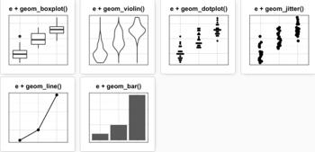
qplot()类似于R基本绘图函数plot(),可以快速绘制常见的几种图形:散点图、箱线图、小提琴图、直方图以及密度曲线图。其绘图格式为:
qplot(x, y=NULL, data, geom="auto")
其中:
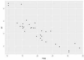
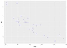
qplot(x=mpg, y=wt, data=df, geom = "point")
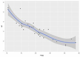
也可以添加平滑曲线
qplot(x=mpg, y=wt, data = df, geom = c("point", "smooth"))
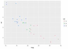
还有其他参数可以修改,比如点的形状、大小、颜色等
#将变量cyl映射给颜色和形状

qplot(x=mpg, y=wt, data = df, colour=cyl, shape=cyl)
#构造数据集
set.seed(1234)
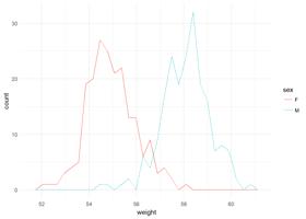
wdata <- data.frame(
sex=factor(rep(c("F", "M"), each=200)),
weight=c(rnorm(200, 55), rnorm(200, 58))
)
head(wdata)
##   sex   weight

## 1   F 53.79293

## 2   F 55.27743

## 3   F 56.08444

## 4   F 52.65430

## 5   F 55.42912

## 6   F 55.50606
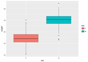
箱线图
qplot(sex, weight, data = wdata, geom = "boxplot", fill=sex)
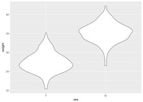
小提琴图
qplot(sex, weight, data = wdata, geom = "violin")
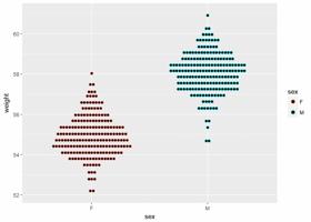
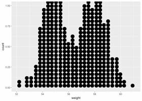
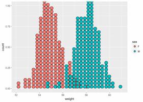
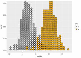
点图
qplot(sex, weight, data = wdata, geom = "dotplot", stackdir="center", binaxis="y", dotsize=0.5, color=sex)
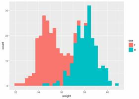
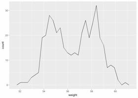
直方图
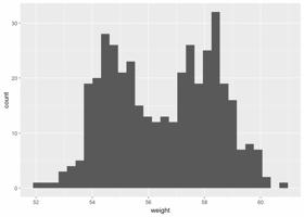
qplot(weight, data = wdata, geom = "histogram", fill=sex)
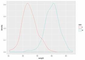
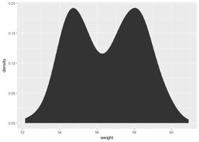
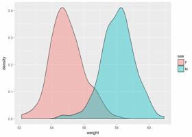
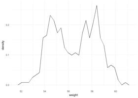
密度图
qplot(weight, data = wdata, geom = "density", color=sex, linetype=sex)
上文中的qplot()绘制散点图:
qplot(x=mpg, y=wt, data=df, geom = "point")
在ggplot()中完全可以如下实现:
ggplot(data=df, aes(x=mpg, y=wt))+

  geom_point()

改变点形状、大小、颜色等属性
ggplot(data=df, aes(x=mpg, y=wt))+geom_point(color="blue", size=2, shape=23)
绘图过程中常常要用到转换(transformation),这时添加图层的另一个方法是用stat_*()函数。
下例中的geom_density()与stat_density()是等价的
ggplot(wdata, aes(x=weight))+geom_density()
等价于
ggplot(wdata, aes(x=weight))+stat_density()
对于每一种几何图形。ggplot2 基本都提供了 geom()和 stat()
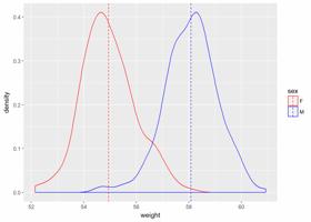
使用数据集wdata,先计算出不同性别的体重平均值
library(plyr)

mu <- ddply(wdata, "sex", summarise, grp.mean=mean(weight))
先绘制一个图层a,后面逐步添加图层
a <- ggplot(wdata, aes(x=weight))
可能添加的图层有:
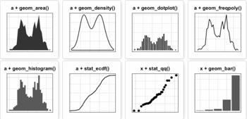
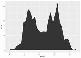
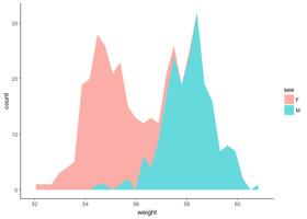
a+geom_area(stat = "bin")
改变颜色
a+geom_area(aes(fill=sex), stat = "bin", alpha=0.6)+

  theme_classic()
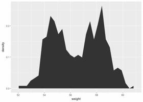
注意:y轴默认为变量weight的数量即count,如果y轴要显示密度,可用以下代码:
a+geom_area(aes(y=..density..), stat = "bin")
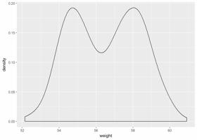
可以通过修改不同属性如透明度、填充颜色、大小、线型等自定义图形:
使用以下函数:
a+geom_density()
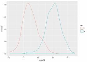
根据sex修改颜色,将sex映射给line颜色
a+geom_density(aes(color=sex))
修改填充颜色以及透明度
a+geom_density(aes(fill=sex), alpha=0.4)
添加均值线以及手动修改颜色
a+geom_density(aes(color=sex))+

  geom_vline(data=mu, aes(xintercept=grp.mean, color=sex), linetype="dashed")+

  scale_color_manual(values = c("red", "blue"))
a+geom_dotplot()
将sex映射给颜色
a+geom_dotplot(aes(fill=sex))
手动修改颜色
a+geom_dotplot(aes(fill=sex))+

  scale_fill_manual(values=c("#999999", "#E69F00"))
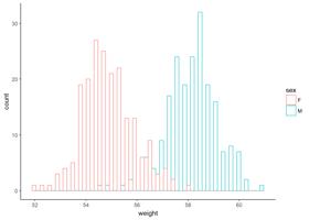
a+geom_freqpoly()
y轴显示为密度
a+geom_freqpoly(aes(y=..density..))+

  theme_minimal()
修改颜色以及线型
a+geom_freqpoly(aes(color=sex, linetype=sex))+

  theme_minimal()
a+geom_histogram()
将sex映射给线颜色
a+geom_histogram(aes(color=sex), fill="white", position = "dodge")+theme_classic()
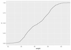
a+stat_ecdf()
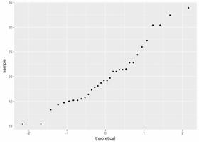
ggplot(data = mtcars, aes(sample=mpg))+stat_qq()
#加载数据集

data(mpg)

b <- ggplot(mpg, aes(x=fl))

b+geom_bar()
修改填充颜色
b+geom_bar(fill="steelblue", color="black")+theme_classic()
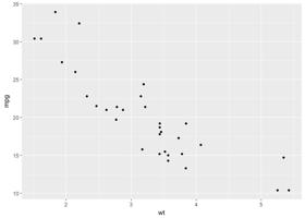
使用数据集mtcars, 先创建一个ggplot图层
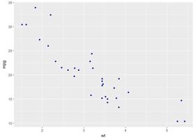
b <- ggplot(data = mtcars, aes(x=wt, y=mpg))
可能添加的图层有:
b+geom_point()
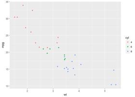
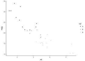
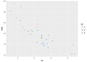
将变量cyl映射给点的颜色和形状
b + geom_point(aes(color = factor(cyl), shape = factor(cyl)))
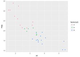
自定义颜色
b+geom_point(aes(color=factor(cyl), shape=factor(cyl)))+

  scale_color_manual(values=c("#999999", "#E69F00", "#56B4E9"))+theme_classic()
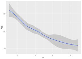
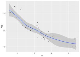
可以添加回归曲线
b+geom_smooth()
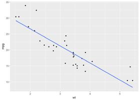
散点图+回归线
b+geom_point()+

  geom_smooth(method = "lm", se=FALSE)#去掉置信区间
使用loess方法
b+geom_point()+

  geom_smooth(method = "loess")
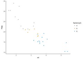
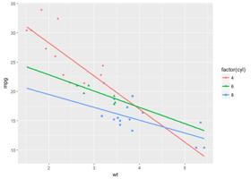
将变量映射给颜色和形状
b+geom_point(aes(color=factor(cyl), shape=factor(cyl)))+

  geom_smooth(aes(color=factor(cyl), shape=factor(cyl)), method = "lm", se=FALSE, fullrange=TRUE)
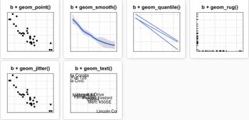
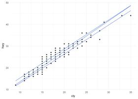
ggplot(data = mpg, aes(cty, hwy))+

  geom_point()+geom_quantile()+

  theme_minimal()
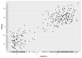
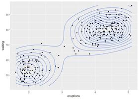
使用数据集faithful
ggplot(data = faithful, aes(x=eruptions, y=waiting))+

  geom_point()+geom_rug()
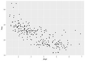
实际上geom_jitter()是geom_point(position=”jitter”)的简称,下面使用数据集mpg
p <- ggplot(data = mpg, aes(displ, hwy))

p+geom_point()
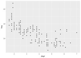
增加抖动防止重叠
p+geom_jitter(width = 0.5, height = 0.5)
其中两个参数:
参数label用来指定注释标签 (ggrepel可以避免标签重叠)
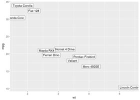
b+geom_text(aes(label=rownames(mtcars)))
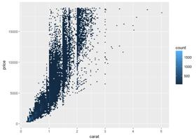
使用数据集diamonds
head(diamonds[, c("carat", "price")])
## # A tibble: 6 x 2

##   carat price

##   <dbl> <int>

## 1  0.23   326

## 2  0.21   326

## 3  0.23   327

## 4  0.29   334

## 5  0.31   335

## 6  0.24   336
创建ggplot图层,后面再逐步添加图层
c <- ggplot(data=diamonds, aes(carat, price))
可添加的图层有:
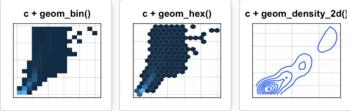
geom_bin2d()将点的数量用矩形封装起来,通过颜色深浅来反映点密度
c+geom_bin2d()
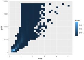
设置bin的数量
c+geom_bin2d(bins=150)
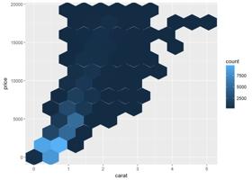
geom_hex()依赖于另一个R包hexbin,所以没安装的先安装:
install.packages("hexbin")
library(hexbin)

c+geom_hex()
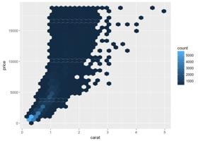
修改bin的数目
c+geom_hex(bins=10)
sp <- ggplot(faithful, aes(x=eruptions, y=waiting))

sp+geom_point()+ geom_density_2d()
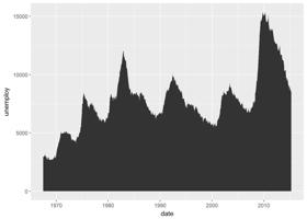
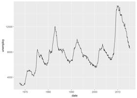
主要是如何通过线来连接两个变量,使用数据集economics。
head(economics)
## # A tibble: 6 x 6

##         date   pce    pop psavert uempmed unemploy

##       <date> <dbl>  <int>   <dbl>   <dbl>    <int>

## 1 1967-07-01 507.4 198712    12.5     4.5     2944

## 2 1967-08-01 510.5 198911    12.5     4.7     2945

## 3 1967-09-01 516.3 199113    11.7     4.6     2958

## 4 1967-10-01 512.9 199311    12.5     4.9     3143

## 5 1967-11-01 518.1 199498    12.5     4.7     3066

## 6 1967-12-01 525.8 199657    12.1     4.8     3018
先创建一个ggplot图层,后面逐步添加图层
d <- ggplot(data = economics, aes(x=date, y=unemploy))
可添加的图层有:
d+geom_area()
d+geom_line()
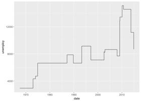
set.seed(1111)

ss <- economics[sample(1:nrow(economics), 20),]

ggplot(ss, aes(x=date, y=unemploy))+

  geom_step()
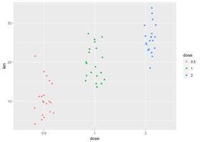
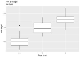
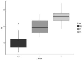
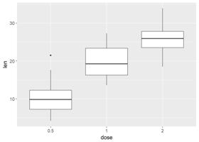
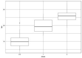
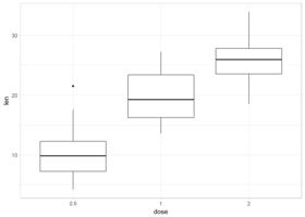
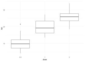
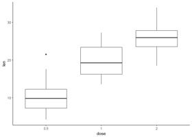
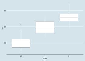
使用数据集ToothGrowth,其中的变量len(Tooth length)是连续变量,dose是离散变量。
ToothGrowth$dose <- as.factor(ToothGrowth$dose)

head(ToothGrowth)
##    len supp dose

## 1  4.2   VC  0.5

## 2 11.5   VC  0.5

## 3  7.3   VC  0.5

## 4  5.8   VC  0.5

## 5  6.4   VC  0.5

## 6 10.0   VC  0.5
创建图层
e <- ggplot(data = ToothGrowth, aes(x=dose, y=len))
可添加的图层有:
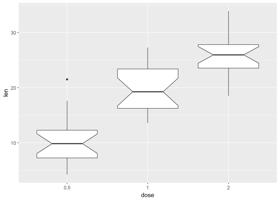
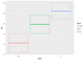
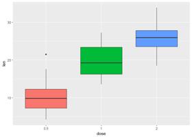
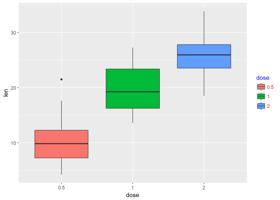
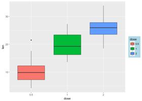
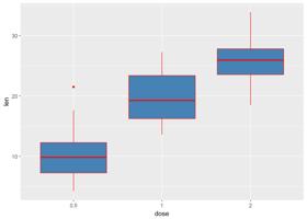
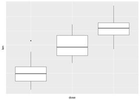
e+geom_boxplot()

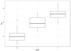
添加有缺口的箱线图
e+geom_boxplot(notch = TRUE)
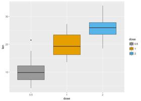
按dose分组映射给颜色
e+geom_boxplot(aes(color=dose))
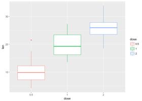
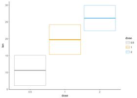
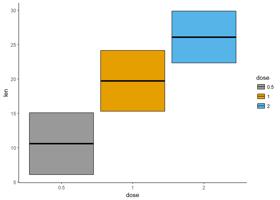
将dose映射给填充颜色
e+geom_boxplot(aes(fill=dose))

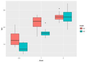
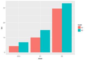
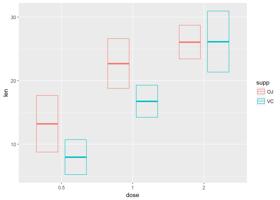
按supp进行分类并映射给填充颜色
ggplot(ToothGrowth, aes(x=dose, y=len))+ geom_boxplot(aes(fill=supp))
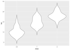
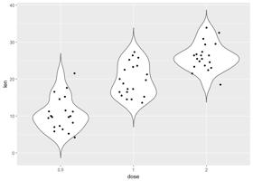
e+geom_violin(trim = FALSE)
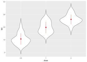
添加中值点
e+geom_violin(trim = FALSE)+

  stat_summary(fun.data = mean_sdl, fun.args = list(mult=1),

               geom="pointrange", color="red")
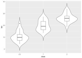
与箱线图结合
e+geom_violin(trim = FALSE)+

  geom_boxplot(width=0.2)
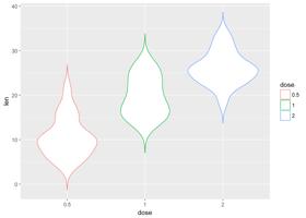
将dose映射给颜色进行分组
e+geom_violin(aes(color=dose), trim = FALSE)
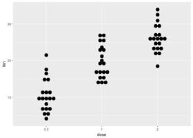
e+geom_dotplot(binaxis = "y", stackdir = "center")
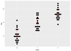
添加中值点
e + geom_dotplot(binaxis = "y", stackdir = "center") +

  stat_summary(fun.data=mean_sdl, color = "red",geom = "pointrange",fun.args=list(mult=1))
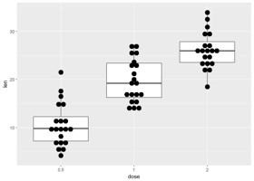
与箱线图结合
e + geom_boxplot() +

  geom_dotplot(binaxis = "y", stackdir = "center")
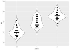
添加小提琴图
e + geom_violin(trim = FALSE) +

  geom_dotplot(binaxis=’y’, stackdir=’center’)
将dose映射给颜色以及填充色
e + geom_dotplot(aes(color = dose, fill = dose),

                 binaxis = "y", stackdir = "center")
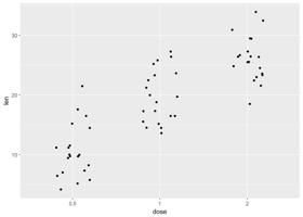
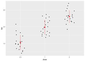
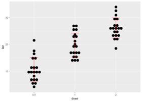
带状图是一种一维散点图,当样本量很小时,与箱线图相当
e + geom_jitter(position=position_jitter(0.2))
添加中值点
e + geom_jitter(position=position_jitter(0.2)) +

  stat_summary(fun.data="mean_sdl",  fun.args = list(mult=1),

               geom="pointrange", color = "red")
与点图结合
e + geom_jitter(position=position_jitter(0.2)) +

  geom_dotplot(binaxis = "y", stackdir = "center")

与小提琴图结合
e + geom_violin(trim = FALSE) +

  geom_jitter(position=position_jitter(0.2))
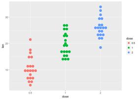
将dose映射给颜色和形状
e +  geom_jitter(aes(color = dose, shape = dose),

                 position=position_jitter(0.2))
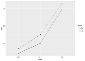
#构造数据集

df <- data.frame(supp=rep(c("VC", "OJ"), each=3),

                dose=rep(c("D0.5", "D1", "D2"),2),

                len=c(6.8, 15, 33, 4.2, 10, 29.5))

head(df)
##   supp dose  len

## 1   VC D0.5  6.8

## 2   VC   D1 15.0

## 3   VC   D2 33.0

## 4   OJ D0.5  4.2

## 5   OJ   D1 10.0

## 6   OJ   D2 29.5
将supp映射线型
ggplot(df, aes(x=dose, y=len, group=supp)) +

  geom_line(aes(linetype=supp))+

  geom_point()
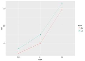
修改线型、点的形状以及颜色
ggplot(df, aes(x=dose, y=len, group=supp)) +

  geom_line(aes(linetype=supp, color = supp))+

  geom_point(aes(shape=supp, color = supp))
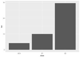
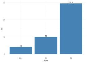
#构造数据集

df <- data.frame(dose=c("D0.5", "D1", "D2"),

                len=c(4.2, 10, 29.5))

head(df)
##   dose  len

## 1 D0.5  4.2

## 2   D1 10.0

## 3   D2 29.5
df2 <- data.frame(supp=rep(c("VC", "OJ"), each=3),

                dose=rep(c("D0.5", "D1", "D2"),2),

                len=c(6.8, 15, 33, 4.2, 10, 29.5))

head(df2)
##   supp dose  len

## 1   VC D0.5  6.8

## 2   VC   D1 15.0

## 3   VC   D2 33.0

## 4   OJ D0.5  4.2

## 5   OJ   D1 10.0

## 6   OJ   D2 29.5
创建图层
f <- ggplot(df, aes(x = dose, y = len))

f + geom_bar(stat = "identity")
修改填充色以及添加标签
f + geom_bar(stat="identity", fill="steelblue")+

  geom_text(aes(label=len), vjust=-0.3, size=3.5)+

  theme_minimal()
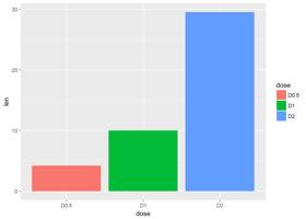
将dose映射给条形图颜色
f + geom_bar(aes(color = dose),

             stat="identity", fill="white")
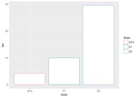
修改填充色
f + geom_bar(aes(fill = dose), stat="identity")
将变量supp映射给填充色,从而达到分组效果
g <- ggplot(data=df2, aes(x=dose, y=len, fill=supp))

g + geom_bar(stat = "identity")#position默认为stack
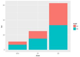
修改position为dodge
g + geom_bar(stat="identity", position=position_dodge())
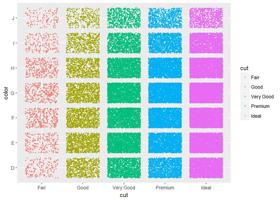
使用数据集diamonds中的两个离散变量color以及cut
ggplot(diamonds, aes(cut, color)) +

  geom_jitter(aes(color = cut), size = 0.5)
df <- ToothGrowth

df$dose <- as.factor(df$dose)

head(df)
##    len supp dose

## 1  4.2   VC  0.5

## 2 11.5   VC  0.5

## 3  7.3   VC  0.5

## 4  5.8   VC  0.5

## 5  6.4   VC  0.5

## 6 10.0   VC  0.5
绘制误差图需要知道均值以及标准误,下面这个函数用来计算每组的均值以及标准误。
data_summary <- function(data, varname, grps){

  require(plyr)

  summary_func <- function(x, col){

    c(mean = mean(x[[col]], na.rm=TRUE),

      sd = sd(x[[col]], na.rm=TRUE))

  }

  data_sum<-ddply(data, grps, .fun=summary_func, varname)

  data_sum <- rename(data_sum, c("mean" = varname))

 return(data_sum)

}
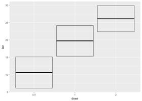
计算均值以及标准误
df2 <- data_summary(df, varname="len", grps= "dose")

# Convert dose to a factor variable

df2$dose=as.factor(df2$dose)

head(df2)
##   dose    len       sd

## 1  0.5 10.605 4.499763

## 2    1 19.735 4.415436

## 3    2 26.100 3.774150
创建图层
f <- ggplot(df2, aes(x = dose, y = len,

                     ymin = len-sd, ymax = len+sd))
可添加的图层有:
具体如下:
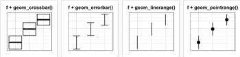
f+geom_crossbar()
将dose映射给颜色
f+geom_crossbar(aes(color=dose))
自定义颜色
f+geom_crossbar(aes(color=dose))+

  scale_color_manual(values = c("#999999", "#E69F00", "#56B4E9"))+theme_classic()
修改填充色
f+geom_crossbar(aes(fill=dose))+

  scale_fill_manual(values = c("#999999", "#E69F00", "#56B4E9"))+

  theme_classic()
通过将supp映射给颜色实现分组,可以利用函数stat_summary()来计算mean和sd
f <- ggplot(df, aes(x=dose, y=len, color=supp))

f+stat_summary(fun.data = mean_sdl, fun.args = list(mult=1), geom="crossbar", width=0.6, position = position_dodge(0.8))
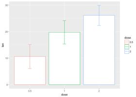
f <- ggplot(df2, aes(x=dose, y=len, ymin=len-sd, ymax=len+sd))
将dose映射给颜色
f+geom_errorbar(aes(color=dose), width=0.2)
与线图结合
f+geom_line(aes(group=1))+

  geom_errorbar(width=0.15)
与条形图结合,并将变量dose映射给颜色
f+geom_bar(aes(color=dose), stat = "identity", fill="white")+

  geom_errorbar(aes(color=dose), width=0.1)
#构造数据集
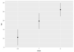
df2 <- data_summary(ToothGrowth, varname="len", grps = "dose")
df2$dose <- as.factor(df2$dose)
head(df2)
##   dose    len       sd

## 1  0.5 10.605 4.499763

## 2    1 19.735 4.415436

## 3    2 26.100 3.774150
创建图层
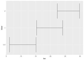
f <- ggplot(data = df2, aes(x=len, y=dose,xmin=len-sd, xmax=len+sd))
参数xmin与xmax用来设置水平误差棒
f+geom_errorbarh()
通过映射实现分组
f+geom_errorbarh(aes(color=dose))
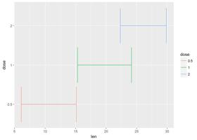
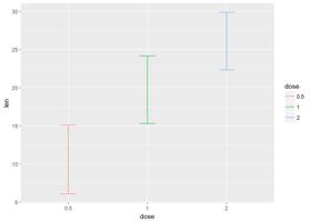
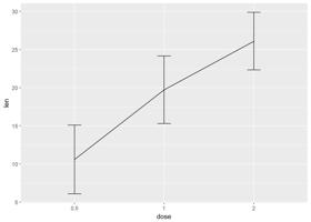
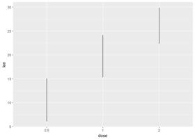
f <- ggplot(df2, aes(x=dose, y=len, ymin=len-sd, ymax=len+sd))
line range
f+geom_linerange()
point range
f+geom_pointrange()
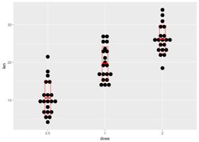
g <- ggplot(df, aes(x=dose, y=len))+

  geom_dotplot(binaxis = "y", stackdir = "center")
添加geom_crossbar()
g+stat_summary(fun.data = mean_sdl, fun.args = list(mult=1), geom="crossbar", color="red", width=0.1)
添加geom_errorbar()
g + stat_summary(fun.data=mean_sdl, fun.args = list(mult=1),

        geom="errorbar", color="red", width=0.2) +

  stat_summary(fun.y=mean, geom="point", color="red")
添加geom_pointrange()
g + stat_summary(fun.data=mean_sdl, fun.args = list(mult=1),

                 geom="pointrange", color="red")

ggplot2提供了绘制地图的函数geom_map(),依赖于包maps提供地理信息。
安装map
install.paclages("maps")
下面将绘制美国地图,数据集采用USArrests
library(maps)

head(USArrests)
##            Murder Assault UrbanPop Rape

## Alabama      13.2     236       58 21.2

## Alaska       10.0     263       48 44.5

## Arizona       8.1     294       80 31.0

## Arkansas      8.8     190       50 19.5

## California    9.0     276       91 40.6

## Colorado      7.9     204       78 38.7
对数据进行整理一下,添加一列state
crimes <- data.frame(state=tolower(rownames(USArrests)), USArrests)

head(crimes)
##            Murder Assault UrbanPop Rape

## Alabama      13.2     236       58 21.2

## Alaska       10.0     263       48 44.5

## Arizona       8.1     294       80 31.0

## Arkansas      8.8     190       50 19.5

## California    9.0     276       91 40.6

## Colorado      7.9     204       78 38.7
#数据重铸

library(reshape2)

crimesm <- melt(crimes, id=1)

head(crimesm)
##        state variable value

## 1    alabama   Murder  13.2

## 2     alaska   Murder  10.0

## 3    arizona   Murder   8.1

## 4   arkansas   Murder   8.8

## 5 california   Murder   9.0

## 6   colorado   Murder   7.9
map_data <- map_data("state")

#绘制地图,使用Murder进行着色

ggplot(crimes, aes(map_id=state))+

  geom_map(aes(fill=Murder), map=map_data)+

  expand_limits(x=map_data$long, y=map_data$lat)

使用数据集mtcars,首先绘制一个相关性图
#构造数据

df <- mtcars[, c(1,3,4,5,6,7)]

head(df)
##                    mpg disp  hp drat    wt  qsec

## Mazda RX4         21.0  160 110 3.90 2.620 16.46

## Mazda RX4 Wag     21.0  160 110 3.90 2.875 17.02

## Datsun 710        22.8  108  93 3.85 2.320 18.61

## Hornet 4 Drive    21.4  258 110 3.08 3.215 19.44

## Hornet Sportabout 18.7  360 175 3.15 3.440 17.02

## Valiant           18.1  225 105 2.76 3.460 20.22
cormat <- round(cor(df), 2)

cormat_melt <- melt(cormat)

head(cormat)
##        mpg  disp    hp  drat    wt  qsec

## mpg   1.00 -0.85 -0.78  0.68 -0.87  0.42

## disp -0.85  1.00  0.79 -0.71  0.89 -0.43

## hp   -0.78  0.79  1.00 -0.45  0.66 -0.71

## drat  0.68 -0.71 -0.45  1.00 -0.71  0.09

## wt   -0.87  0.89  0.66 -0.71  1.00 -0.17

## qsec  0.42 -0.43 -0.71  0.09 -0.17  1.00
创建图层:
g <- ggplot(cormat_melt, aes(x=Var1, y=Var2))
在此基础上可添加的图层有:
现在使用使用geom_tile()绘制相关性矩阵图,我们这里这绘制下三角矩阵图,首先要整理数据:
#获得相关矩阵的下三角

get_lower_tri <- function(cormat){

  cormat[upper.tri(cormat)] <- NA

  return(cormat)

}

#获得相关矩阵的上三角

get_upper_tri <- function(cormat){

  cormat[lower.tri(cormat)] <- NA

  return(cormat)

}

upper_tri <- get_upper_tri(cormat = cormat)

head(upper_tri)
##      mpg  disp    hp  drat    wt  qsec

## mpg    1 -0.85 -0.78  0.68 -0.87  0.42

## disp  NA  1.00  0.79 -0.71  0.89 -0.43

## hp    NA    NA  1.00 -0.45  0.66 -0.71

## drat  NA    NA    NA  1.00 -0.71  0.09

## wt    NA    NA    NA    NA  1.00 -0.17

## qsec  NA    NA    NA    NA    NA  1.00
绘制相关矩阵图
#数据重铸

upper_tri_melt <- melt(upper_tri, na.rm = TRUE)

ggplot(data=upper_tri_melt, aes(Var1, y=Var2, fill=value))+

  geom_tile(color="white")+

  scale_fill_gradient2(low = "blue", high = "red", mid = "white", midpoint = 0, limit=c(-1, 1), space = "Lab", name="Person

Correlation")+

  theme_minimal()+

  theme(axis.text.x = element_text(angle = 45, vjust = 1, size = 12, hjust = 1))+

  coord_fixed()
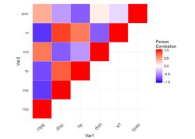
上图中蓝色代表互相关,红色代表正相关,至于coord_fixed()保证x,y轴比例为1
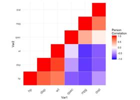
可以看出上图顺序有点乱,我们可以对相关矩阵进行排序
#构造函数

reorder_cormat <- function(cormat){

  dd <- as.dist((1-cormat)/2)

  hc <- hclust(dd)

  cormat <- cormat[hc$order, hc$order]

}

cormat <- reorder_cormat(cormat)

lower_tri <- get_lower_tri(cormat)

lower_tri_melt <- melt(lower_tri, na.rm = TRUE)

head(lower_tri_melt)
##   Var1 Var2 value

## 1   hp   hp  1.00

## 2 disp   hp  0.79

## 3   wt   hp  0.66

## 4 qsec   hp -0.71

## 5  mpg   hp -0.78

## 6 drat   hp -0.45
绘制图形
ggheatmap <- ggplot(lower_tri_melt, aes(Var1, Var2, fill=value))+

  geom_tile(color="white")+

  scale_fill_gradient2(low = "blue", high = "red", mid = "white", midpoint = 0, limit=c(-1, 1), space = "Lab", name="Person

Correlation")+

  theme_minimal()+

 theme(axis.text.x = element_text(angle = 45, vjust = 1,

    size = 12, hjust = 1))+

 coord_fixed()

print(ggheatmap)
本节主要讲述的是添加图形元件,将用到一下函数:
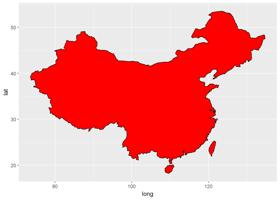
library(dplyr)

map_data("world")%>%

  filter(region==c("China", "Taiwan"))%>%

  ggplot(aes(x=long, y=lat, group=group))+

  geom_polygon(fill="red", color="black")
创建图层
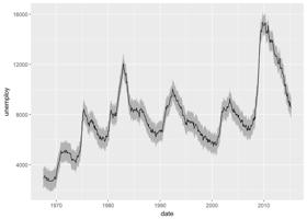
h <- ggplot(economics, aes(date, unemploy))
添加路径
h+geom_path()

添加带状
h+geom_ribbon(aes(ymin=unemploy-800, ymax=unemploy+800), fill = "grey70")+geom_line(aes(y=unemploy))
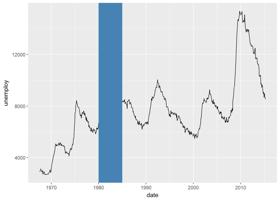
添加矩形
h+

  geom_path()+

  geom_rect(aes(xmin=as.Date("1980-01-01"), ymin=-Inf, xmax=as.Date("1985-01-01"), ymax=Inf), fill="steelblue")
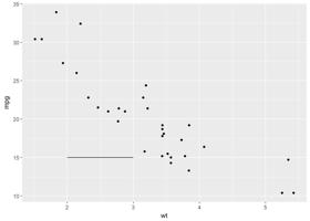
i <- ggplot(mtcars, aes(wt, mpg))+geom_point()

#添加线段

i+geom_segment(aes(x=2, y=15, xend=3, yend=15))
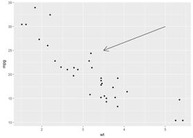
添加箭头
i+geom_segment(aes(x=5, y=30, xend=3.5, yend=25), arrow = arrow(length = unit(0.5, "cm")))
i+geom_curve(aes(x=2, y=15, xend=3, yend=15), color="red")
创建图层
ToothGrowth$dose <- as.factor(ToothGrowth$dose)

p <- ggplot(ToothGrowth, aes(x=dose, y=len))+geom_boxplot()
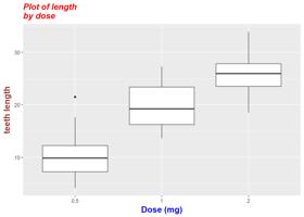
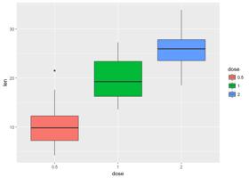
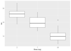
修改标题以及标签的函数有:
(p <- p+labs(title="Plot of length

by dose", x="Dose (mg)", y="teeth length"))
使用theme()修改,element_text()可以具体修改图形参数,element_blank()隐藏标签
#修改标签

p+theme(

plot.title = element_text(color = "red", size = 14, face = "bold.italic"),

axis.title.x = element_text(color="blue", size = 14, face = "bold"),

axis.title.y = element_text(color="#993333", size = 14, face = "bold")

)
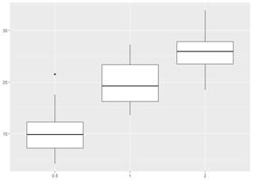
#隐藏标签

p+theme(

  plot.title = element_blank(),

  axis.title.x = element_blank(),

  axis.title.y = element_blank()

)
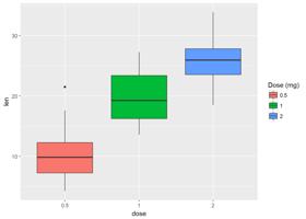
p <- ggplot(ToothGrowth, aes(x=dose, y=len, fill=dose))+

  geom_boxplot()

p
#修改图例标题

p+labs(fill="Dose (mg)")
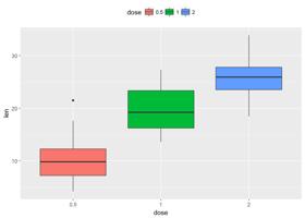
#图例位置在最上面,有五个选项:"left","top", "right", "bottom", "none"

p+theme(legend.position = "top")
移除图例
p+theme(legend.position = "none")
修改图例标题以及标签外观
p+theme(

  legend.title = element_text(color="blue"),

  legend.text = element_text(color="red")

)
修改图例背景
p+theme(legend.background = element_rect(fill="lightblue"))
主要两个函数:
#修改顺序
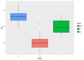
p+scale_x_discrete(limits=c("2", "0.5", "1"))
#修改标题以及标签
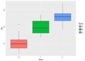
p+scale_fill_discrete(name="Dose", label=c("A","B","C"))
mtcars$cyl <- as.factor(mtcars$cyl)
创建图层
# boxplot

bp <- ggplot(ToothGrowth, aes(x=dose, y=len))

# scatter plot

sp <- ggplot(mtcars, aes(x=wt, y=mpg))
bp+geom_boxplot(fill="steelblue", color="red")
sp+geom_point(color="darkblue")
(bp <- bp+geom_boxplot(aes(fill=dose)))

(sp <- sp+geom_point(aes(color=cyl)))
主要两个函数:
# Box plot

bp + scale_fill_manual(values=c("#999999", "#E69F00", "#56B4E9"))
# Scatter plot

sp + scale_color_manual(values=c("#999999", "#E69F00", "#56B4E9"))
# Box plot

bp + scale_fill_brewer(palette="Dark2")

# Scatter plot

sp + scale_color_brewer(palette="Dark2")
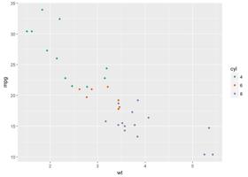
RColorBrewer包提供以下调色板
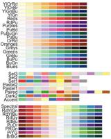
还专门有一个灰度调色板:
# Box plot

bp + scale_fill_grey() + theme_classic()
# Scatter plot

sp + scale_color_grey() + theme_classic()
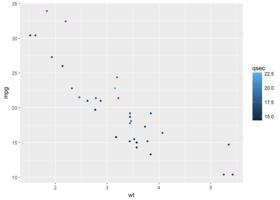
有时我们会将某个连续变量映射给颜色,这时修改这种梯度或连续型颜色就可以使用以下函数:
# Color by qsec values

sp2<-ggplot(mtcars, aes(x=wt, y=mpg)) +

  geom_point(aes(color = qsec))

sp2
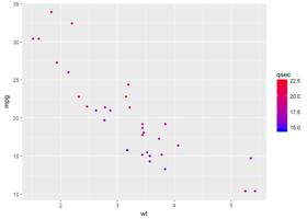
# Change the low and high colors

# Sequential color scheme

sp2+scale_color_gradient(low="blue", high="red")
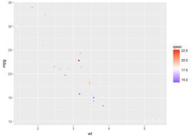
# Diverging color scheme

mid<-mean(mtcars$qsec)

sp2+scale_color_gradient2(midpoint=mid, low="blue", mid="white",

                          high="red", space = "Lab" )
R提供的点形状是由数字表示的,具体如下:

# Basic scatter plot

ggplot(mtcars, aes(x=wt, y=mpg)) +

  geom_point(shape = 18, color = "steelblue", size = 4)
# Change point shapes and colors by groups
ggplot(mtcars, aes(x=wt, y=mpg)) +
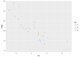
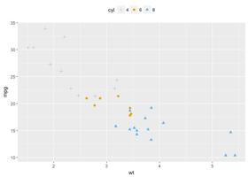
geom_point(aes(shape = cyl, color = cyl))
可通过以下方法对点的颜色、大小、形状进行修改:
# Change colors and shapes manually

ggplot(mtcars, aes(x=wt, y=mpg, group=cyl)) +

  geom_point(aes(shape=cyl, color=cyl), size=2)+

  scale_shape_manual(values=c(3, 16, 17))+

  scale_color_manual(values=c(’#999999’,’#E69F00’, ’#56B4E9’))+

  theme(legend.position="top")
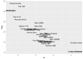
对图形进行文本注释有以下方法:
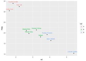
set.seed(1234)

df <- mtcars[sample(1:nrow(mtcars), 10), ]

df$cyl <- as.factor(df$cyl)
散点图注释
# Scatter plot

sp <- ggplot(df, aes(x=wt, y=mpg))+ geom_point()

# Add text, change colors by groups

sp + geom_text(aes(label = rownames(df), color = cyl),

               size = 3, vjust = -1)
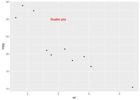
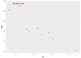
# Add text at a particular coordinate

sp + geom_text(x = 3, y = 30, label = "Scatter plot",

              color="red")
# geom_label()进行注释

sp + geom_label(aes(label=rownames(df)))
# annotation_custom(),需要用到textGrob()

library(grid)

# Create a text

grob <- grobTree(textGrob("Scatter plot", x=0.1,  y=0.95, hjust=0,

  gp=gpar(col="red", fontsize=13, fontface="italic")))

# Plot

sp + annotation_custom(grob)
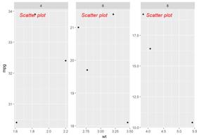
#分面注释

sp + annotation_custom(grob)+facet_wrap(~cyl, scales="free")
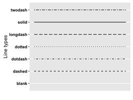
R里的线型有七种:“blank”, “solid”, “dashed”, “dotted”, “dotdash”, “longdash”, “twodash”,对应数字0,1,2,3,4,5,6.
具体如下:
# Create some data

df2 <- data.frame(sex = rep(c("Female", "Male"), each=3),

                  time=c("breakfeast", "Lunch", "Dinner"),

                  bill=c(10, 30, 15, 13, 40, 17) )

head(df2)
##      sex       time bill

## 1 Female breakfeast   10

## 2 Female      Lunch   30

## 3 Female     Dinner   15

## 4   Male breakfeast   13

## 5   Male      Lunch   40

## 6   Male     Dinner   17
# Line plot with multiple groups
# Change line types and colors by groups (sex)
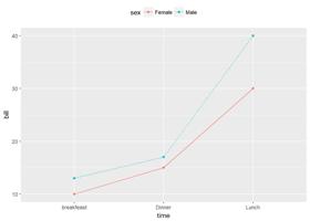
ggplot(df2, aes(x=time, y=bill, group=sex)) +
geom_line(aes(linetype = sex, color = sex))+
geom_point(aes(color=sex))+
theme(legend.position="top")
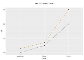
同点一样,线也可以类似修改:
# Change line types, colors and sizes

ggplot(df2, aes(x=time, y=bill, group=sex)) +

  geom_line(aes(linetype=sex, color=sex, size=sex))+

  geom_point()+

  scale_linetype_manual(values=c("twodash", "dotted"))+

  scale_color_manual(values=c(’#999999’,’#E69F00’))+

  scale_size_manual(values=c(1, 1.5))+

  theme(legend.position="top")
# Convert the column dose from numeric to factor variable

ToothGrowth$dose <- as.factor(ToothGrowth$dose)
创建箱线图
p <- ggplot(ToothGrowth, aes(x=dose, y=len))+

  geom_boxplot()
修改主题
ggplot2提供了好几种主题,另外有一个扩展包ggthemes专门提供了一主题,可以安装利用。
install.packages("ggthemes")
p+theme_gray(base_size = 14)
p+theme_bw()
p + theme_linedraw()
p + theme_light()
p + theme_minimal()
p + theme_classic()
ggthemes提供的主题
p+ggthemes::theme_economist()
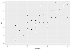
p <- ggplot(cars, aes(x=speed, y=dist))+geom_point()
修改坐标轴范围有以下几种方式:
1、不删除数据
2、会删除部分数据:不在此范围内的数据都会被删除,因此在此基础上添加图层时数据是不完整的
3、扩展图形范围:expand()函数,扩大范围
下面通过图形演示
p

#通过coord_cartesian()函数修改坐标轴范围

p+coord_cartesian(xlim =c (5, 20), ylim = c(0, 50))

#通过xlim()和ylim()函数修改

p+xlim(5, 20)+ylim(0, 50)
#expand limits

p+expand_limits(x=c(5, 50), y=c(0, 150))
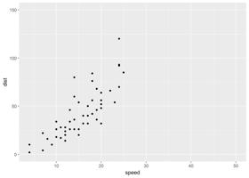
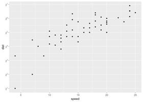
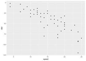
p <- ggplot(cars, aes(x=speed, y=dist))+geom_point()
坐标变换有以下几种:
下面实例演示:
p
p+scale_x_continuous(trans = "log2")+

  scale_y_continuous(trans = "log2")
#修改坐标刻度标签

require(scales)

p+scale_y_continuous(trans=log2_trans(),

                     breaks = trans_breaks("log2", function(x) 2^x),

                     labels=trans_format("log2", math_format(2^.x)))

#坐标轴反向

p+scale_y_reverse()
更改坐标轴刻度线标签等函数:
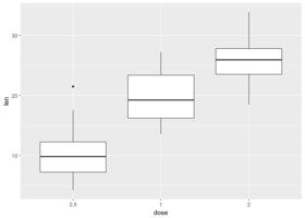
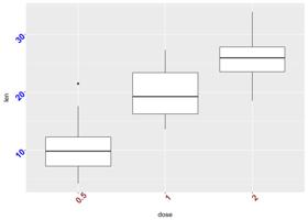
(p <- ggplot(ToothGrowth, aes(x=dose, y=len))+geom_boxplot())
修改刻度标签等
p+theme(axis.text.x = element_text(face = "bold", color="#993333", size=14, angle = 45),

        axis.text.y = element_text(face = "bold", size = 14, color = "blue", angle = 45))
移除刻度标签等
p + theme(

  axis.text.x = element_blank(), # Remove x axis tick labels

  axis.text.y = element_blank(), # Remove y axis tick labels

  axis.ticks = element_blank()) # Remove ticks
当然可以自定义坐标轴了
详细情况如下:
其中scale_xx()函数可以修改坐标轴的如下参数:
具体演示:
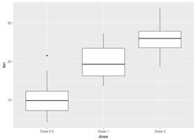
#修改标签以及顺序

p+scale_x_discrete(name="Dose (mg)", limits=c("2", "1", "0.5"))
#修改刻度标签

p+scale_x_discrete(breaks=c("0.5", "1", "2"),labels=c("Dose 0.5", "Dose 1", "Dose 2"))
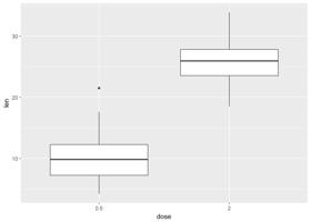
#修改要显示的项

p+scale_x_discrete(limits=c("0.5", "2"))
实例演示:
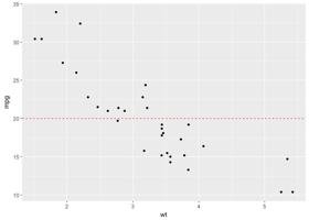
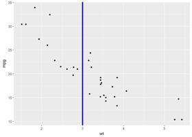
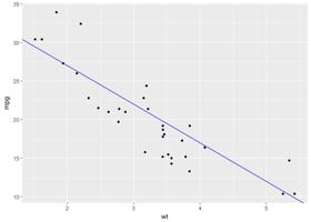
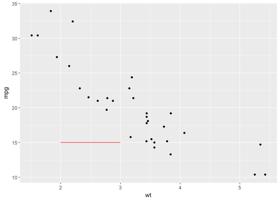
sp <- ggplot(data=mtcars, aes(x=wt, y=mpg))+ geom_point()
添加直线:
#在y=20处添加一水平线,并设置颜色等

sp+geom_hline(yintercept = 20, linetype="dashed", color=’red’)
#在x=3处添加一竖直线,并设置颜色等

sp+geom_vline(xintercept = 3, color="blue", size=1.5)
#添加回归线
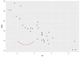
sp+geom_abline(intercept = 37, slope = -5, color="blue")
#添加水平线段

sp+geom_segment(aes(x=2, y=15, xend=3, yend=15), color="red")
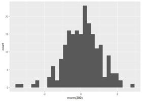
主要是下面两个函数:
set.seed(1234)

(hp <- qplot(x=rnorm(200), geom = "histogram"))
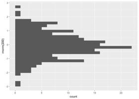
#水平柱形图

hp+coord_flip()
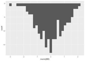
#y轴反向

hp+scale_y_reverse()
分面就是根据一个或多个变量将图形分为几个图形以便于可视化,主要有两个方法实现:
ToothGrowth$dose <- as.factor(ToothGrowth$dose)

(p <- ggplot(ToothGrowth, aes(x=dose, y=len, group=dose))+

  geom_boxplot(aes(fill=dose)))

针对上面图形进行分面:
1、按一个离散变量进行分面:
#竖直方向进行分面

p+facet_grid(supp~.)

#水平方向分面

p+facet_grid(.~supp)
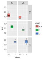
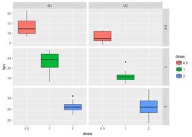
2、按两个离散变量进行分面
#行按dose分面,列按supp分面

p+facet_grid(dose~supp)

#行按supp,列按dose分面

p+facet_grid(supp~dose)
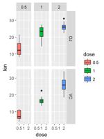
从上面图形可以看出,每个面板的坐标轴比例都是一样的,我们可以通过设置参数scales来控制坐标轴比例
p + facet_grid(dose ~ supp, scales=’free’)
很多图形需要我们调整位置,比如直方图时,由堆叠式、百分式、分离式等,具体的要通过实例说明
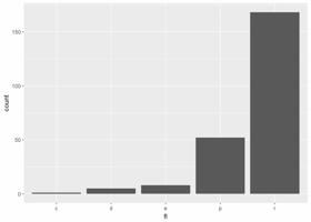
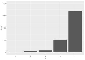
p <- ggplot(mpg, aes(fl, fill=drv))

#直方图边靠边排列,参数position="dodge"

p+geom_bar(position = "dodge")
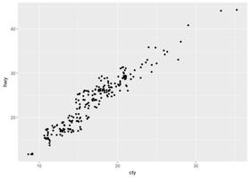
ggplot(mpg, aes(cty, hwy))+

  geom_point(position = "jitter")
上面几个函数有两个重要的参数:heigth、weight。
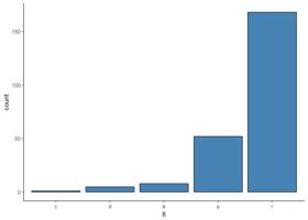
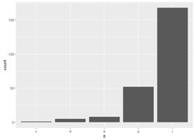
p+geom_bar(position = position_dodge(width = 1))
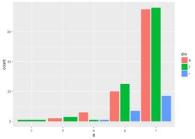
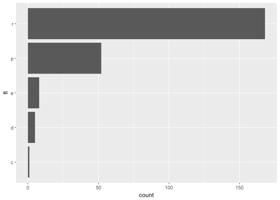
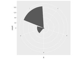
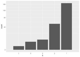
p <- ggplot(mpg, aes(fl))+geom_bar()
ggplot2中的坐标系主要有:
各个坐标系参数如下:
1、笛卡尔坐标系:coord_cartesian(), coord_fixed() and coord_flip()
2、极坐标系:coord_polar()
3、变换坐标系:coord_trans()
实例演示:
p+coord_cartesian(ylim = c(0,200))
p+coord_fixed(ratio = 1/50)
p+coord_flip()
p+coord_polar(theta = "x", direction = 1)
p+coord_trans(y="sqrt")
以上就是关于gg游戏修改器找脚本_gg修改器怎样执行游戏脚本的全部内容,希望对大家有帮助。

gg修改器免root什么用,gg修改器免root的实用性 大小:19.89MB9,620人安装 近年来,越来越多的手机游戏的出现让人们的生活更加多彩。但有时,我们在玩手机游戏……
下载
GG修改器最新破解版,gg游戏修改器破解版免费下载 大小:14.54MB11,184人安装 GG修改器最新破解版,gg游戏修改器破解版免费下载 1、配置临时文件的路径 ①按“ 设置……
下载
gg修改器32位中文版下载,gg修改器怎么改32位 大小:3.04MB11,092人安装 gg修改器是一款功能强大使用简单的手机端数据修改器软件通过这款软件用户可以方便的……
下载
修改器游戏修改器下载GG,GG修改器-给你打造游戏王者之路 大小:3.67MB9,883人安装 在如今这个游戏红利不断升级的时代,越来越多的人加入了游戏热潮。随着玩家的不断增……
下载
华为gg修改器免root版,华为GG修改器免Root版:为你带来无限乐趣 大小:15.32MB9,541人安装 华为GG修改器免Root版是一个非常实用、功能强大的工具。在这个讲究游戏体验的时代,……
下载
gg游戏修改器苹果版下载,为您推荐最佳游戏体验gg游戏修改器苹果版下载 大小:16.35MB9,515人安装 在玩游戏时,不免会遇到一些难以克服的关卡,这时候,游戏修改器就会让您拥有更好的……
下载
gg修改器最新版8.40,令人欣喜的gg修改器最新版8.40 大小:5.50MB9,704人安装 对于游戏玩家来说,gg修改器是一个非常重要的软件工具。它能够修改游戏内的数据,使……
下载
类似于gg的游戏修改器推荐,类似于GG的游戏修改器简介 大小:16.70MB9,723人安装 GG游戏修改器是目前很受欢迎的游戏修改器之一,不过它只适用于安卓系统。对于苹果用……
下载
gg修改器99.0中文版_gg修改器99.0官方版本 大小:10.90MB10,863人安装 大家好,今天小编为大家分享关于gg修改器99.0中文版_gg修改器99.0官方版本的内容,……
下载
gg游戏修改器中文下载,闪亮登场的GG游戏修改器中文下载 大小:9.52MB9,661人安装 如果你是一名游戏爱好者,那么一定会遇到一些让你感到困惑的问题,比如游戏难度太大……
下载